In distributed database systems in general, as well as in the system that zen8labs is implementing, replication and partitioning (also known as sharding) are two crucial techniques to ensure availability and scalability. My article will help you to gain a better understanding of partitioning and how to apply them in an effective manner. 

Partitioning and replication

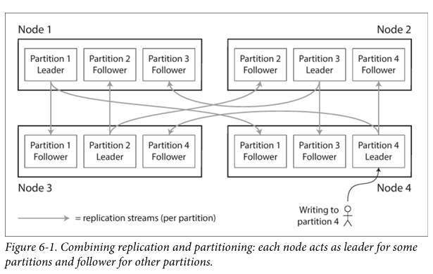
Replication is the process of creating multiple copies of the same data on different nodes. This enhances fault tolerance and ensures that data is always available even if one node fails. In a leader-follower model, each partition has a leader responsible for writing data and followers that replicate from the leader to ensure consistency. 

While replication involves having multiple copies of the same data on different nodes, it may not suffice for very large datasets or high query throughput requirements. In such cases, data needs to be split into partitions (shards). 

Typically, each piece of data (record, row, document) belongs to exactly one partition. Each partition operates like a small independent database, although the system can support operations across multiple partitions simultaneously. 

The main purpose of partitioning is Scalability. Partitioning helps: 

• Data distribution: Breaking large data into smaller partitions and distributing them across multiple disks. 
• Query load distribution: Sending queries to different nodes, increasing the overall throughput of the system. 
• Increased parallel processing: Complex queries can be executed in parallel across multiple nodes. 

Partitioning of key-value data

When dealing with a large amount of data and wanting to partition it, how do you decide which nodes to store records on? 

The purpose of partitioning is to distribute both data and query load evenly across nodes. 

Example: Suppose each node receives an equal amount of data and queries; with 10 nodes, our system can handle 10 times the data and 10 times the read/write throughput compared to a single node. 

If partitioning is uneven, some partitions may have more data or be queried more frequently than others—this is called skewed partitioning. In the worst case, all the load might be concentrated on one partition, known as a hot spot. 

The simplest way to avoid hot spots is to assign records to nodes randomly. This helps distribute data fairly evenly across nodes, but it has a major drawback: when trying to read a specific data item, there’s no way to know exactly which node to access, so you have to query all nodes in parallel. 

Partitioning by key range

Another way to partition is to assign a continuous range of keys (from a minimum value to a maximum) to each partition. If you know the boundaries between ranges, you can easily determine which partition contains a specific key. If you also know which partition is assigned to which node, you can send requests directly to the appropriate node. 

Example: In an encyclopedia dataset, each volume contains a continuous range of letters, such as volume 1 includes words starting with A and B, while volume 12 contains words starting with T, U, V, X, Y, and Z. This makes it easy to determine which volume contains the word you are looking for without having to check all volumes. 

Key ranges do not necessarily need to be evenly distributed but should adapt to the data so that data can be distributed evenly. For instance, one volume of the encyclopedia might contain words starting with A-B, while another contains words starting with T-Z. 

Partition boundaries can be manually selected by the administrator or automatically by the database. 

Disadvantage: Range-based partitioning can lead to hot spots if certain access patterns cause a concentration of data in specific partitions. 

Example: Suppose the key is a timestamp (e.g., year-month-day-hour-minute-second), and you assign one partition per day. If you are writing sensor data to the database as measurements occur, all records for today will go into the same daily partition, overloading that partition while others remain inactive. 

Solution: To avoid this issue in sensor databases, use an element other than the timestamp as the first part of the key. For example, prepend the sensor name to each timestamp to first partition by sensor name and then by time (e.g., sensor1-2024-04-27). 

Partitioning by hash of key

Due to the risk of skewing and creating hot spots, many distributed storage systems use a hash function to determine the partition for certain keys. A good hash function will transform uneven data into a uniform distribution. For example, with a 32-bit hash function taking in a string, each new string will produce a random number in the range from 0 to 2³²−1. Even if the input strings are very similar, their hash values will be uniformly distributed across this range. 

For partitioning purposes, the hash function does not need to be cryptographically strong. For example, Cassandra and MongoDB use MD5, while Voldemort uses the Fowler-Noll–Vo hash function. 

Once a suitable hash function is in place, each partition can be assigned a specific range of hash values. Any key whose hash value falls within this range will be stored in the corresponding partition. This technique helps distribute keys evenly among partitions and can use either evenly sized partition boundaries or choose them randomly (known as consistent hashing). 

Advantages: 

• Even data distribution: Reduces the risk of creating hot spots. 
• Easy scalability: Adding or removing partitions requires moving minimal data. 

Disadvantages: 

• Poor range query performance: Keys that were previously closed are now scattered across partitions, losing their order. For example, in MongoDB with hash-based partitioning, any range query must be sent to all partitions. 
• Limited support for secondary queries: Systems like Riak, Couchbase, and Voldemort do not support range queries on primary keys effectively. 

Cassandra’s approach: Cassandra balances hash-based partitioning with efficient range queries by allowing a composite primary key consisting of multiple columns: 

• The first part of the key is hashed to determine the partition. 
• The remaining columns are used as a sequential index to sort data within Cassandra’s SSTables. 

This sequential indexing approach allows for flexible data modeling for one-to-many relationships. For example, on a social networking site, a user may post many updates. If the primary key for updates is chosen as (user_id, update_timestamp), you can efficiently retrieve all updates from a user within a time range, sorted by timestamp. Different users can be stored in different partitions, but within each user, updates are stored in timestamp order within a single partition. 

Skewed workloads and relieving hot spots 

Hashing a key to determine its partition can help reduce hot spots. However, it cannot completely eliminate them: in the worst case where all read/write operations target the same key, you still have to send all requests to a single partition. 

Example: On a social networking site, a famous user with millions of followers might generate a storm of activity when they perform an action. This event could lead to a large number of writes to the same key (the key might be the celebrity’s user ID or an action ID that others are commenting on). Hashing the key does not help, as the hash of identical IDs remains the same. 

Current Solutions: Most data systems cannot automatically adjust for such highly skewed loads, so the responsibility to mitigate this skew lies with the application. For example, if you know a key is very hot, a simple technique is to append or prepend a random number to the key. Just adding a two-digit random number can spread writes across 100 different keys, allowing these keys to be distributed to different partitions. 

Disadvantages: 

• Complex reads: When writes are spread across multiple keys, any reader must retrieve data from all 100 keys and combine them, increasing latency. 
• Complex management: This technique only makes sense when applied to a small number of hot keys. For most low-write-volume keys, adding random numbers would introduce unnecessary overhead. 
• Need to monitor hot keys: To apply this effectively, the application must have mechanisms to track and identify keys being split, ensuring that only genuinely hot keys are subject to this technique. 

Partitioning and secondary indexes 

The partitioning schemes discussed so far rely on a key-value data model. If records are only ever accessed via their primary key, we can determine the partition from that key and use it to route read and write requests to the partition responsible for that key. 

However, the situation becomes more complex when secondary indexes are involved. Secondary indexes often do not uniquely identify records but are a way to search for specific values: find all actions of user 123, find all posts containing the word “hogwash,” find all cars with red color, etc. 

Secondary indexes are foundational in relational databases and are also popular in document databases. Many key-value systems (like HBase and Voldemort) have avoided using secondary indexes due to the complexity of implementation, but some systems (like Riak) have started adding them because they are very useful for data modeling. Ultimately, secondary indexes are the reason search servers like Solr and Elasticsearch exist. 

The problem with secondary indexes is that they do not fit neatly with partitioning. There are two main methods to distribute a database with secondary indexes: 

1. Document-based distribution 
2. Term-based distribution 

Partitioning secondary indexes by document 

Example: Imagine operating a used car website (as illustrated in Figure 6-4). Each car listing has a unique ID—let’s call it the document ID—and we partition the database by that document ID (e.g., IDs from 0 to 499 go to partition 0, IDs from 500 to 999 go to partition 1, etc.). 

The website allows users to search for cars with filters like color and manufacturer, so secondary indexes on these attributes need to be created. If we have declared an index, the database can perform indexing automatically. For example, whenever a red car is added to the database, the partition automatically adds its document ID to the list for the color:red index. 

In this indexing method, each partition is completely independent and maintains its own secondary indexes, related only to the documents within that partition. Whenever there is a change in the database, only the partition containing that document ID needs to be involved. For this reason, partitioned-by-document indexes are also known as local indexes (as opposed to global indexes, described in the next section). 

Disadvantage

Reading from a document-partitioned index requires care. Unless you have done something special with document IDs, there is no reason why all cars of the same color or manufacturer would reside within the same partition. In Figure 6-4, red cars appear in both partition 0 and partition 1. Therefore, if you want to search for red cars, you need to send queries to all partitions and combine all returned results. 

When searching for documents based on a secondary index (e.g., all red cars), the system must send queries to all partitions and merge the results (scatter/gather), leading to increased latency and resource consumption. However, this method is widely used: MongoDB, Riak, Cassandra, Elasticsearch, SolrCloud, and VoltDB all use document-partitioned secondary indexes. Most database vendors recommend structuring the partitioning scheme so that secondary index queries can be served from a single partition, but this is not always possible, especially when using multiple secondary indexes in a single query (for example, filtering cars by both color and manufacturer simultaneously). 

Partitioning secondary indexes by term 

Instead of each partition having its own index (local index), we can build a global index that covers data across all partitions. However, this global index should not be stored on a single node, as it could become a bottleneck. A global index also needs to be partitioned, but differently from the primary key index. 

Example: In a global index, red cars from all partitions are listed under color:red, and this index is partitioned based on the first letter of the color: from A to R go to partition 0, and from S to Z go to partition 1. Similarly, the index for the car manufacturer is also partitioned based on the first letter of the manufacturer’s name. 

This type of index is called a term-partitioned index, as the search terms determine the index’s partitioning. The “term” here is similar to words in text indexes, as in search engines. 

As before, we can partition the index based on the term itself or use a hash of the term: 

• Partition by term itself: Useful for range searches, such as car prices. 
• Partition by hash of term: Provides a more even load distribution. 

Advantages of global indexes (Term-partitioned): 

• Faster Reads: Instead of performing scatter/gather across all partitions, we only need to query the partition containing the desired term. 

Disadvantages of global indexes: 

• Slower and more complex writes: A write operation to a single document might affect multiple index partitions (all terms in the document could be in different partitions, on different nodes). 

Index updates: In an ideal world, indexes are always updated immediately as changes occur in the database. In reality, global secondary index updates often occur asynchronously. This means that after writing data, the index may not be updated immediately. For example, Amazon DynamoDB updates global secondary indexes within a fraction of a second under normal conditions but may experience delays during infrastructure issues. 

Rebalancing partitions 

Why rebalancing is important 

As a database system grows, many changing factors need to be managed: 

• Increase in users: More users will increase query load on the database, requiring us to add CPU resources to handle it. 
• Increase in data size: We need to add more disks and RAM to store larger data. 
• Server failures: If a server fails, other servers must take over the responsibilities of the failed node. 

These changes require data and request movements from one machine to another within the cluster. This process is called rebalancing. Rebalancing needs to meet the following requirements: 

• Even load distribution: The workload is evenly distributed among nodes. 
• System availability: The rebalancing process does not disrupt service. 
• Minimal data movement: Minimize the amount of data that needs to be moved to save resources. 

Strategies for rebalancing 

Avoid using hash mod N

When partitioning data by hashing keys, we typically divide hash values into ranges and assign each range to a specific partition. A simple method is to use modulo hashing (hash(key) mod N), for example, hash(key) mod 10 to assign keys to 10 nodes numbered 0 to 9. 

However, when the number of nodes changes, most keys will need to be moved to new nodes. For instance, with hash(key) mod 10, adding an 11th node means most keys need to be moved from node 6 to node 3 (hash(key) mod 11). 

Continuous movement like this makes the rebalancing process expensive and complex. 

Fixed number of partitions

A simple way to manage partitioning is to create more partitions than the current number of nodes and assign multiple partitions to each node. For example, with 10 nodes in the cluster, you can create 1,000 partitions, with each node responsible for approximately 100 partitions. 

Balancing when adding or removing nodes: 

• Adding a new node: The new node takes some partitions from existing nodes to redistribute evenly. 
• Removing a node: The partitions of the removed node are transferred to the remaining nodes. 

Only the new partitions are moved between nodes. The number of partitions and how keys are assigned to partitions do not change. During the transition, the system still uses the old partition assignment method to handle read and write requests. 

We can assign more partitions to more powerful nodes to have them handle more load, helping to balance the load based on each node’s hardware capabilities. 

This method is used in systems like Riak, Elasticsearch, Couchbase, and Voldemort. 

Choosing the number of partitions: The number of partitions is typically fixed at initialization and does not change later, which makes management easier. However, choosing this number is challenging when the data size changes significantly. Therefore, the initial number of partitions needs to be carefully selected to appropriately support future growth and avoid increased management costs. 

Dynamic partitioning 

For databases using range-based partitioning, setting a fixed number and boundaries of partitions often faces many difficulties. If boundaries are chosen poorly, all data might concentrate in one partition while others remain empty. Manually adjusting partition boundaries is time-consuming and laborious. 

To address this, databases like HBase and RethinkDB implement dynamic partitioning. This method automatically splits a partition when data exceeds a limit and merges it when data drops below a certain threshold. 

Each partition is assigned to a node in the system, and partitions can be moved between nodes to balance the load. This helps the number of partitions automatically adjust according to data volume: fewer partitions when data is low, and more partitions when data is large. 

Initial partitioning: When a new database is created, it starts with a single partition. This can lead to bottlenecks as data grows, but systems like HBase and MongoDB support pre-splitting partitions to minimize this issue, requiring users to know the partition key distribution in advance. 

Dynamic partitioning suits both range-based partitioning and hash-based partitioning (MongoDB from version 2.4 supports both types of partitioning). 

Partitioning proportionally to nodes 

In dynamic partitioning, the number of partitions increases or decreases with data size as partitions are split or merged to maintain a stable partition size. Conversely, with a fixed number of partitions, each partition’s size grows with the data. In both cases, the number of partitions does not depend on the number of nodes in the system. 

Another approach: Cassandra and Ketama make the number of partitions proportional to the number of nodes—meaning each node has a fixed number of partitions. When data increases, each partition’s size grows, but when adding new nodes, partitions are split, helping to maintain partition sizes consistently. This is suitable when large data volumes require more nodes for storage. 

Adding a new node: When a new node joins the cluster, it randomly selects some existing partitions to split. The new node then takes half of the data from each split partition, while the other half remains on the old node. This process can lead to uneven splits, but when there are many partitions (e.g., Cassandra defaults to 256 partitions per node), the distribution becomes fairer. 

Partition boundaries: Choosing random partition boundaries requires using hash-based partitioning, allowing boundaries to be selected from the range generated by the hash function. This method is analogous to the original definition of consistent hashing. Modern hash functions can achieve similar effectiveness with lower metadata costs. 

Conclusion

Through a deep dive into the replication and partitioning strategies utilized in distributed database systems, we’ve explored the vital roles these techniques play in enhancing system availability, fault tolerance, and scalability. This discussion has not only highlighted the fundamental principles of partitioning but also showcased various methods and their implementations, underscoring their importance in managing and distributing large data sets efficiently. 

As we’ve seen, the choice of partitioning strategy can significantly impact the performance and manageability of a database. Whether through range-based, hash-based, or dynamic partitioning, each method offers unique benefits and comes with its set of challenges. By understanding these nuances and applying the appropriate partitioning strategy, organizations can ensure that their database systems are robust, scalable, and capable of handling increasing loads and complex query requirements. 

Looking forward, the continuous evolution of data needs and system architectures will likely bring new challenges to the forefront of database management. In response, engineers and developers must remain agile, ready to adapt and innovate partitioning strategies to meet these changing demands. At zen8labs, we are committed to pioneering advanced solutions that tackle these issues, helping our clients to not only meet but exceed their data handling expectations. 

I hope I have showed you the benefits that partitioning can have for you moving forward. Now if you want to find out some more insightful things my colleagues and I do at zen8labs, then click here! 

Hieu Ngoc Ha, Software Engineer